Building Image Classification Models Based on Pre-Trained Neural Networks

Introduction

The era of AI democratization is already here. The number of pre-trained APIs, algorithms, development and training tools that help data scientist build the next generation of AI-powered applications is only growing.

There are already a big number of models that were trained by professionals with a huge amount of data and computational power. Many of such models are open-source, so anyone can use them for their own purposes free of charge. Being able to use these models effectively is one of the key skills of a competent data scientist.

In this article, I will try to show the benefits of using pre-trained models and will explain how you can adapt them to a specific image classification task.

For this purpose, I chose LifeCLEF2014 Plant Identification Task as a demo case.

Image Classification Task Description

We will try to predict a taxonomical class of a plant based on multi-image plant observations. There are 47815 plant images available for training, each image belongs to one of 500 plant species. The goal is to predict the correct plant species among the top results of a ranked list of species returned by our image classification system. The final score is related to the rank of the correct species in the list of predicted species.

Constraints imposed by organizers forbid using any additional information including pre-trained models.

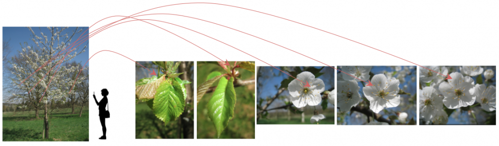
The image classification task simulates a real scenario where a user tries to identify a plant by observing its different parts (stem, leaf, flower) the same day with the same device with the same lighting conditions, as demonstrated in the picture below. Thus, the task won’t be image-centered but observation-centered.

Since the quality and the number of images observed by different contributors varies, organizers have suggested a metric that will evaluate the ability of a system to provide correct answers to all users. So, the primary quality metric is defined as the following average classification score S:

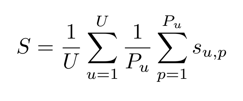
• U : number of users (who have at least one image in the test data)
• Pu : number of individual plants observed by the u-th user
• Su,p : score between 1 and 0 equals to the inverse of the rank of the correct species (for the p-th plant observed by the u-th user).

Our Approach

The contest has very strict limitations, but in the real life, we are free to use any available sources of information and pre-built tools. In particular, for solving this image classification problem we decided to break the rule set by the organizers, use pre-trained neural networks and show multiple advantages of this approach.

We will use neural networks that were trained on 1.2 million images from ImageNet with 1000 different object categories, such as computer, plane, table, cat, dog and other simple objects we encounter in our day-to-day lives. We have selected VGG16, VGG19, ResNet50, InceptionV3 as the basic neural networks. Since these models have been trained on a huge amount of images and have already learned information about very general simple objects, there is a hope that they can help us create a better system for our image classification task.

So, let’s start from … image preprocessing, of course.

Image Preprocessing

Preprocessing is based on the idea of selecting the most important part of an image. We will rely on the methods that were used by the winner of the competition (IBM Research team) making some minor changes.

Each image in the dataset is associated with metadata: author, view content (content), average vote of users (whether an image is good for classification or not), latitude and longitude of place where a photo has been taken and other. We focus on the visual part of the dataset, for that reason the ‘Content’ field is the most important for us.

There are seven values for ‘view content’: Entire, Branch, Flower, Fruit, LeafScan, Leaf, Stem. We will use a specific preprocessing method for each ‘view content’.

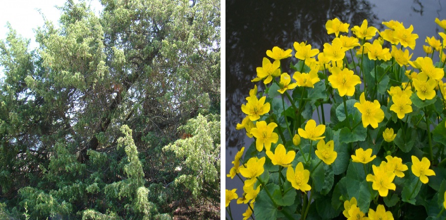
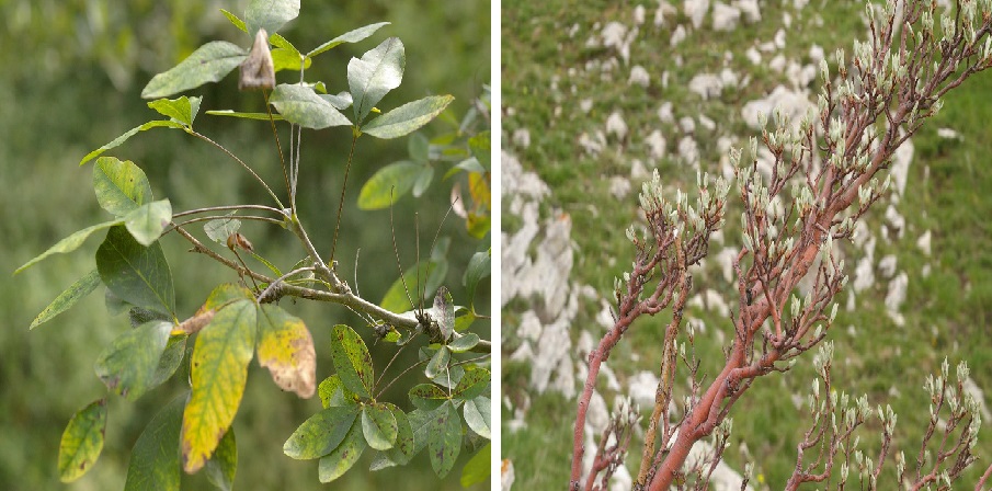
Entire and Branch

We won’t change Entire or Branch photographs, as they may contain useful information, that we don’t want to lose.

Examples of Entire:

Examples of Branch:

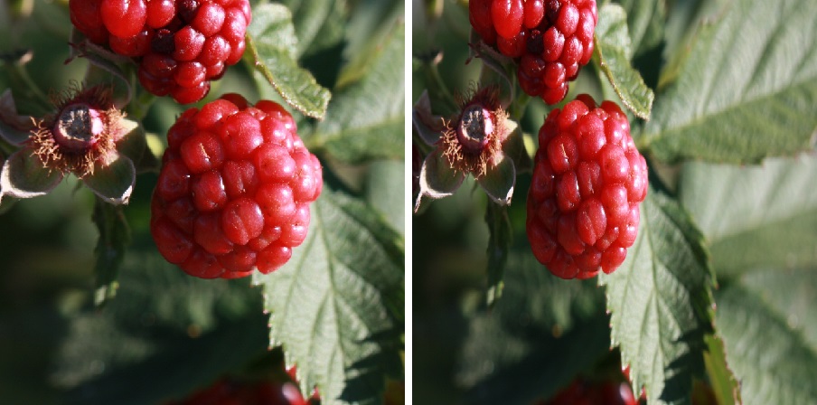
Flower and Fruit

For Flower and Fruit images we will use a similar preprocessing method:

• convert a photo into a grayscale image;
• use Gaussian filter with parameter a = 2.5;
• apply active contour method to find most important part of the photo;
• compute a minimum bounding box.

Example of Flower preprocessing:

Example of Fruit preprocessing:

LeafScan

Looking through the photographs of LeafScan type, you can notice that there is usually a leaf with a light background. We will normalize an image with the white color:

• first, we convert a color image into a grayscale image and use Otsu method to compute a threshold;
• after that, all pixels that have a value that is less than a computed threshold are assigned with a white color.

Example of LeafScan preprocessing:

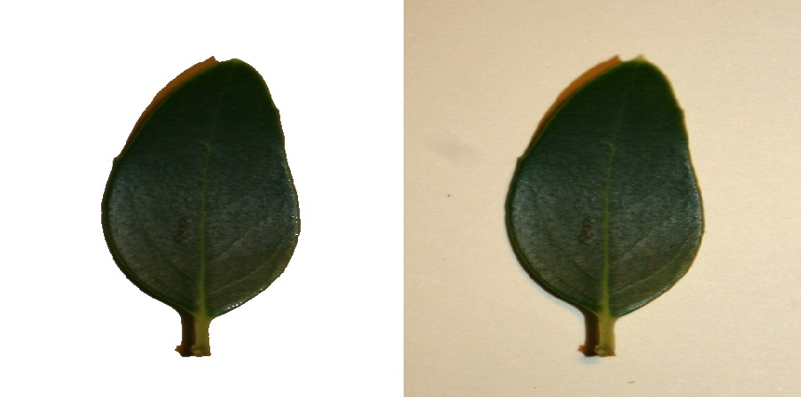
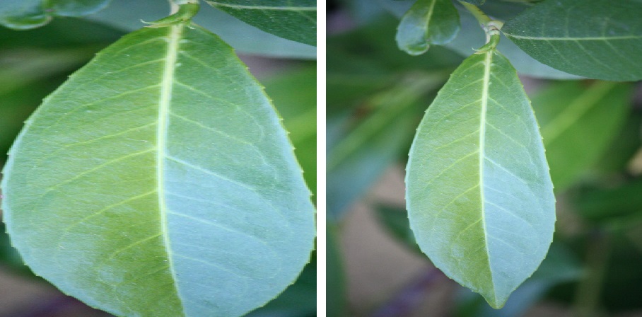
Leaf

Typically Leaf images contain leaves that are located in the center of the image with some padding between the contour of a leaf and the border of the picture. So our preprocessing algorithm is as follows:

• we cut 1/10 of an image in all directions: left, right, bottom, top without losing essential details;
• after that, we convert the color picture into a grayscale image;
• use Gaussian filter with parameter a = 2;
• apply active contour method to compute a minimal bounding box.

Example of Leaf preprocessing:

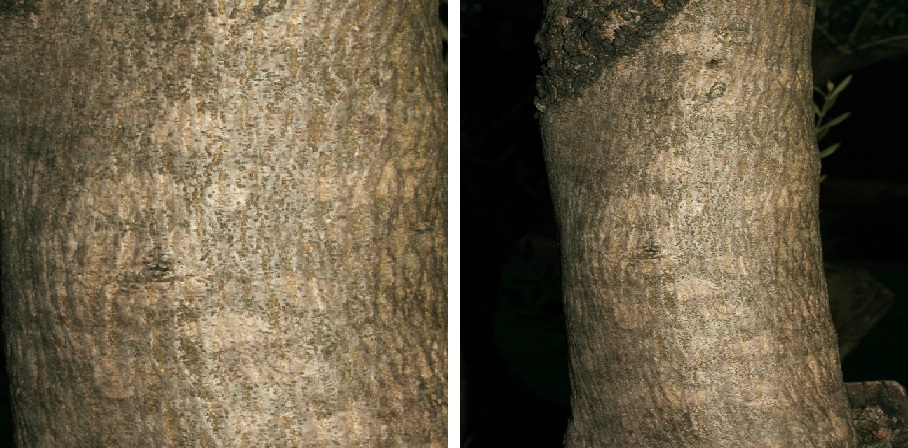
Stem

In Stem photographs, stem is usually located in the center of an image. Out steps:

• we can safely cut ⅕ of an image in all directions: left, right, bottom, top;
• apply Gaussian filter with a = 2;
• convert a color image into a grayscale picture;
• finally, use active contour method to compute a minimal bounding box.

Example of Stem preprocessing:

Now everything is ready for building our image classification model. We will use Keras with TensorFlow backend. It’s a powerful machine learning library for neural networks that allows a lot of things from building simple models like perceptron to creating really complex networks that can deal with video. And most importantly, Keras provides an opportunity to use pre-trained neural networks and allows us to optimize models with both CPU and GPU.

3 Steps to Build Image Classification Models Using Pre-Trained Neural Networks:

1. Using the Bottleneck Features of a Pre-trained Neural Network

Initially, we import a pre-trained neural network without dense layers and apply pooling to its output. Average pooling (GlobalAveragePooling) works better than maximum pooling in our case.

Then we run this model on our training data and save the output in a file. Later you will see why we need to do so.

2. Training Dense Model Based on Bottleneck Features

We could freeze convolutional blocks of a pre-trained model and add our neural network on top of it, but we won’t do that because in this case, we will need to predict output for every image for each epoch, which will take quite a lot of time. Time is a finite resource, so in order to save some we will use the features that we saved before, and train the dense model on top of them.

At this step, we also need to split training data into training and validation datasets. For example in the ratio 3 : 1.

Now let’s take a closer look at the dense network that we are going to train. After some experiments we have discovered that one of the best architectures has the following structure:

• 3 dense layers with 512 neurons, each of them is followed by a dropout with parameter 0.5, which means that we randomly switch off half of the neurons to avoid overfitting;
• the output layer is softmax for 500 classes;
• we use categorical cross-entropy as a loss function and optimize our network with Adam;
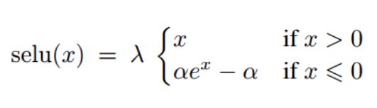
• we have found out that using selu (scaled exponential unit) for dense layers instead of traditional relu allows our network to converge faster.

Note that:

• for the described training method we can’t use augmentation (transformations of images, e.g. rotation, zooming, adding noise), but the model that we get is just the first approximation to the final classifier, so it’s not a problem for us;
• these neural networks are trained quickly, so we can manually set a required number of epochs;
• overfitting is not a big problem as well because we will be able to fix it later;
• it takes from 40 to 80 epochs for the neural networks to converge.

3. Combining Models into Final Image Classification System

At this step, we add our previously trained dense model on top of the pre-trained neural network. We change the optimizer while the loss function remains the same.

The pre-trained network has learned a lot of abstract and general features, so in order not to wreck the previously learned features we start training the whole thing, with a very slow learning rate. Optimizers like Adam and RMSProp are adaptive learning rate optimizers, which doesn’t meet our needs. I recommend using SGD-optimizer because it allows us to keep the magnitude of the updates small.

In Order to Build a Powerful Image Classification Model, Keep in Mind that:

• you should reduce learning rate on the plateau (using ReduceLROnPlateau callback), in order not to go to a minimum too fast.
• you should stop training a model (using EarlyStopping callback) when validation loss has not been improving for several epochs.
• you should save training information in a file after each epoch (using CSVLogger callback), so that we could track and analyze how the training of a network goes. Typically fine-tuning takes a lot of time and when we close .ipynb-files we lose all the dynamic output.

For nice progress bars, I like using TQDMNotebookCallback, rather than the standard one in Keras. It doesn’t influence the final result but makes the work more pleasant.

Data Augmentation

When fine-tuning the entire network, we can use augmentation. But instead of using standard ImageDataGenerator from Keras we use Imgaug, which is a powerful library for image augmentation. A very important feature of Imgaug is that it allows us to explicitly define a probability that transformation will be applied, we can also create a group of transformations and choose which set to apply.

We choose transformations that can happen in real life, such as horizontal flipping, rotation, zooming, different contrast, brightness, and noise. It is important not to apply all possible transformations at the same time as it would be hard for the neural network to learn features and converge.

It is better to split transformations into several groups and apply each of them with a specified probability. Uncommonly we will augment image only in 80%, which means that with probability p = 0.2 we don’t change an input image so that neural network could see the real one.

Leverage User Ratings on Image Quality

Each image in the dataset has a vote annotation (an average of the user ratings on image quality). We noticed that images with vote 1 or 2 are very noisy, and though they contain some useful information they may disserve our final model. We tested the hypothesis while training the neural networks based on InceptionV3. There are very few images with vote 1 (only 1966 images), so we tried to delete them from the training set. The network trained better without the images with vote 1, so I encourage you to experiment more with this hypothesis.

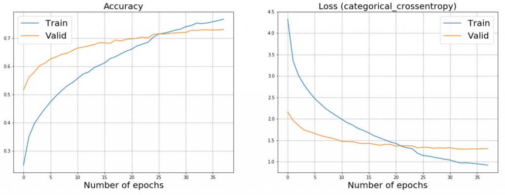
You can see the plots of ResNet50 and InceptionV3 fine-tuning below. Jumping ahead a bit, I should say that we achieved the best results with these models that is why I provide them as examples.

Plot of fine-tuning ResNet50:

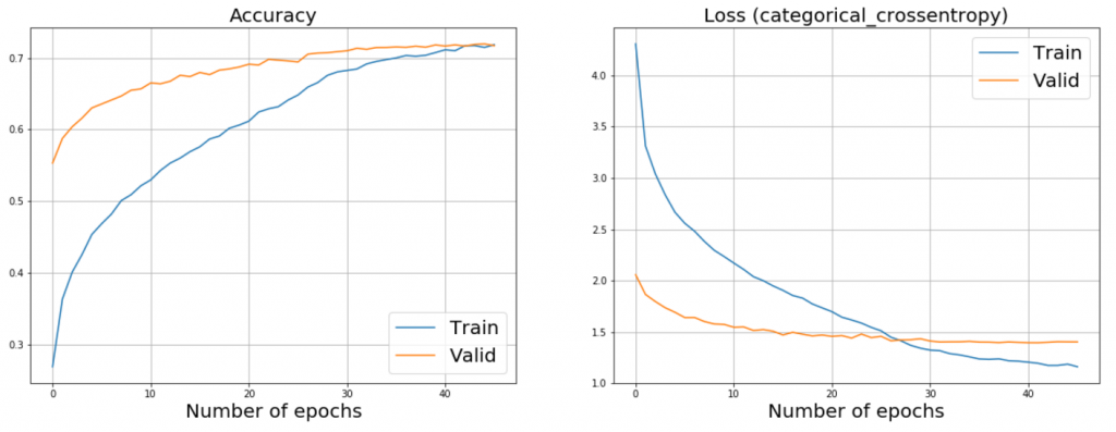
Plot of fine-tuning InceptionV3:

Test-time Augmentation

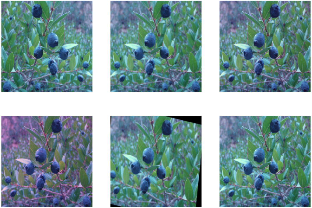
Another thing that helped me to improve quality is test-time augmentation (TTA). I suggest you predicting output not only for a test image but also for some augmented versions of the image. For example, we can take 5 most realistic augmentations, apply them to the image and make predictions on 6 images, rather than using only one image. After that, we take an average prediction as a final output. !!! Note that you should use only one transformation at a time for test image augmentation.

Example of test-time augmentation:

Results

You can find the results of our research in the table below.

Let’s compare the following metrics: primary metric S, that was provided by organizers and 3 versions of top metrics – Top1, Top3, Top5. Top metrics are used for each observation (a set of images of the same plant), but not for each image.

We also tried to merge several models to explore if it can help us improve the results (when merging models we took the average prediction). The last three rows in the table show results of these merged models.

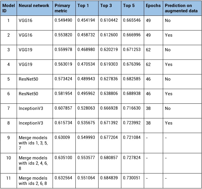
The best system built by the winner of the competition achieved a validation accuracy of 0.471 (primary metric). Their system is a fusion of statistical methods and neural network and doesn’t use pre-trained neural networks.

Our classification method that uses a pre-trained neural network as a base model, reaches an accuracy of 0.60785, achieving a 29% relative improvement over the winning entry of the contest.

When we use test-time data augmentation, the primary metric improves up to 0.615734 but at the same time, the speed of the model drops significantly (the model works 6 times slower).

By merging outputs of several neural networks we can improve results even further. This method gets us to an accuracy of 0.635100 but reduces the speed dramatically and in the real life can be applied only to a laboratory research when the speed is not a priority.

Existing models are not 100% accurate, and sometimes when we meet an unknown plant, it can be helpful to know a list of the most probable species of the plant. Here we can use top-n metric, which reflects an accuracy of a model in predicting the correct species among top-n most probable species. A fine-tuned neural network that uses one image for prediction reaches an accuracy of 0.716630 for Top 5 metric. The accuracy improves to 0.730051 when we use augmented data for predictions.

I described how to achieve better quality using pre-trained neural networks, but it’s not the only way for improvement. I’d like to encourage you not to stop here and to try a few more approaches to improve your image classification model:

• more accurate image pre-processing
• modification of architecture of a dense model
• change the activation function (or its hyperparameters)
• use images of the best quality for training (images with vote greater than 2)
• explore the distribution of classes in the training dataset to and use class_weights parameter for training

Conclusion

Fine-tuning neural networks that were originally trained on more than 1 million pictures made it possible to significantly outperform the best solution of the contest. Our approach has proved that pre-trained models can be very helpful for image classification tasks, especially in situations when you don’t have a big enough dataset. Even if the base model is not directly connected to your problem it still can be very helpful since it has already learned to recognize simple objects.

To recap, here are my top tips to achieve better results:

• Use Imgaug for data augmentation (it allows more transformations comparing with Keras ImageDataGenerator);
• During the training, apply augmentation with probability 0.8 instead of traditional 1;
• Use test-time augmentation (take an average of the predictions on augmented data);
• Reduce learning rate on plateau;
• Stop training if validation loss doesn’t improve for several epochs;
• Train your model on images with vote greater than 1.

I wish you good luck with your experiments! If you have any comments about this post or if you need help with your computer vision project, you can contact our team at info@indatalabs.com.

P.S. I’d like to thank my team for their help, the research and the article wouldn’t be possible without them. Thanks to Dzianis Pirshtuk who put me in charge of the research. Thanks to Denis Dus and Alexey Tishurov for their expert advice and mentorship. And many thanks to Irina Peregud for helping me edit and publish the article.

The cover image courtesy the artist Shinseungback Kimyonghun.