Imagine, you have a camera observable environment. What can you do with data from the cameras besides just recording videos for security reasons? What can you do with images taken by mobile cameras? Many things. Even if your production or product is not related to cameras. Production surveillance automation, smart car camera security systems, fitness exercises assessment, automated counterfeit fighting, paper documents digitization – these are just a few examples of possible projects which may be powered with computer vision.
And if the project can be decomposed into standard computer vision problems, like object detection, keypoint estimation, image classification, semantic segmentation, metric learning etc., then it can be done – because most known computer vision problems have years – even dozens of years of studies, so there are known ways to solve them.
Problems Formulation for Computer Vision
In simple words computer vision is solving vision tasks with the help of computers. Visions tasks have input (image) and output (decision, based on image content). Regarding output structure there are such task like:
| Task | Output structure |
|---|---|
| Object detection – find all ‘interesting’ objects on image | Position and size of bounding boxes for each object of interest on image |
| Semantic segmentation – find exactly ‘interesting’ part of image | For each pixel on image: whether it belongs to the area of interest or not |
| Human Pose Estimation – understand human pose based on image | Grouped by person location of each skeleton joint and other key points (if needed) on image |
| Image classification – decide whether an image, by some criteria, falls in one of the classes of interests or not | Label of class to which image belongs |
What Does Computer Vision Offer for Business?
Take a look at a few examples of applying computer vision problem formulation for business problems.
Surveillance on Production Environments
A very common problem for industrial production environments is understanding whether employees respect security measures or not. For example, on construction or quarry one of such important security measures is protective equipment usage. Enforcement of such measures can be done with hiring operators to watch videos from multiple security cameras. This may be too costly, though.

Source: Unsplash
Can we reduce current expenses on such surveillance needs? Yes. We can do it through automation.
Business problem: to reduce the number of actual surveillance employees keeping security standards.
Solution: computer vision-based automation, or, more specifically, an auto alert when an employee violates protective equipment usage rules.
We can pick out from this problem two particular subproblems:
- Find each employee on video frames
- Understand, whether each employee uses protective equipment in a proper way or not
Formally, these are computer vision problems: object detection (object is human) and image classification (classify each detected person image as violating rules or not). These tasks are to be solved by data scientists with computer vision expertise.
Prerequisite is to collect a large dataset of rule violation and compliance examples and label it with help of data labeling specialists.
The above mentioned decomposition has the potential to reuse already existing person detectors and only spend time for creating employee classification models. But applying different strategies, it is possible to expect better accuracy in detection security violation events. For example, one can build a single model which not only detects employees but simultaneously performs classification (e.g. detect three classes of objects – just a person, employee violating security rules, employee non-violating security rules). Or even, approach can be not to create classification models, but create a detector of persons and each class of protective equipment with further rule based decision on security rules violation.
Following such kinds of problems, computer vision solutions may help businesses to reduce expenses keeping security standards.
Incident Management
The International Labour Organization states that 2.3 million workers succumb to workplace accidents and diseases every year. That makes over 6000 deaths per day. Today, computer vision aims to advance occupational safety and health (OSH), minimize the workers’ exposure to various risk factors, and detect early signs of impending hazards.
Computer vision models learn to recognize hazards from massive image data sets. The more data they study, the better the results. Over the time, they recognize hazards as good as EHS managers (Environment, health and safety) do. Moreover, CV-enabled software can monitor sites 24/7, while humans can’t. If the software detects abnormalities, a safety manager gets an alert and goes to the site to intervene. That makes AI workplace safety solutions beneficial for occupational safety.
Pose Estimation for Workout Assessment
Smart devices with cameras surround us everywhere. Smartphones, tablets, laptops – most of them are equipped with cameras. One of the applications of such cameras aiming not only at entertainment but health and wellbeing is automatic assessment of fitness exercises correctness. Real-time workout assessment is achieved with pose estimation technology.

Source: Unsplash
The classic of fitness training is to be guided by a trainer at some fitness club. But easily accessible camera-equipped devices allow ones to create automated solutions for these purposes.
Consider, a business task is to create a mobile application for yoga asanas training. Computer vision surely can help us here. Each yoga asana is a special human pose, so formally we are talking about human pose estimation problems with further pose classification. Following such kinds of problems, computer vision solutions may help businesses provide solutions for healthy life.
Well, it seems computer vision may help business with many challenges, but how do all these computer solutions work? Shoot a frame, perform some kind of magic, and provide a result? Actually, the general pipeline looks almost so, but it is not magic underlying, just applied math.
General Concepts for Computer Vision Problems Solving
Computer vision challenges can be solved in many ways. Before 2015 prevalent methods were to use so-called “classic computer vision” techniques: combination of classic machine learning algorithms (like logistic regression, neural networks, random forest, SVM) with handcrafted image based features (obtained using digital image processing algorithms). In 2012 deep neural networks started to beat classical computer vision in some tasks, and after 2015 deep neural networks became state of the art for solving many computer vision tasks. So, regardless of talking about classic computer vision or deep learning based, machine learning is key for both.
Machine Learning
Machine learning is, in some sense, a math application for automatic building decision models using real world data. At the beginning non-trained machine learning models connect their inputs with their outputs randomly. When we use machine learning algorithms to fit the model to the data (train model) we aim to determine exactly one way to connect inputs with outputs from all possible ways, so that at least for given test ground truth data on input outputs are as close to ground truth outputs as possible.
Just to highlight what this “as close” means, consider we have a detection model with two classes – protective helmet and protective vest. Depending on this model trained or not, possible model outputs for input helmet image are:
| Model | Output (class “probability”) |
|---|---|
| Not trained | 50% helmet, 50% vest (random output) |
| Trained, correct answer | 90% helmet, 10% vest |
| Trained, error happened | 40% helmet, 60% vest |
| Ground truth | 100% helmet, 0% vest |
In the table you can see the row where an “error happened”. Unfortunately, when one deals with machine learning – errors may happen. And a great part of machine learning work is focused on making a particular model as accurate as possible. Moreover, the automatic process of fitting any model to the properly prepared data is itself an iterative reduction of model error. The difference between algorithmic and manual work is that model fitting algorithm fits a model to a subset of data called training set. A specialist enforces that model to perform accurately on non-seen by model during fitting process data called test set and also on the model usage time. One of simplest and widespread machine learning models is logistic regression.
Logistic Regression
It is one of the simplest machine learning models. Consider, some real world objects can be described by some number of values (N numbers) – features. For example, a building can be described by number of rooms, total area, number of floors, presence of electricity or gas.
A logistic regression model has parameters called weights for each of input variables, these weights mean how much contribute each input variable for model output. For example, if we want to build a prediction model for whether a building is living or not, model output will show the probability that the building is living. Parameters of the models is a subject of the model training algorithm. Our simple model of living building prediction in case of logistic regression will be in next form:

Sigmoid in formula is a function often used in machine learning, this function compresses it’s input into a (0; 1) interval. Like on next image:
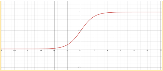
Because we use real world data for model training, then a trained model is a model of some real world dependencies. The thing is – most dependencies in the real world are non-linear. It means that output cannot be represented as a linear combination of inputs. Or, in other words, it means there is no separating hyperplane for different data point groups in the original space of inputs. But many of the models are still linear. How then, can they deal with non linear data?
Non Linearity Handling
Before model application machine learning specialist develops features that may project initially non linear data into space where data becomes almost linear.
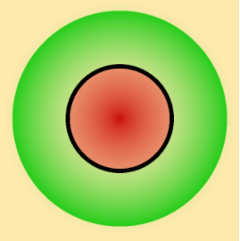
Just as an example (trivial, but well understandable): imagine you have some hazard source in production and want to have a model which predicts danger according to the position on a two-dimensional map, like is that point safe or not. Ground truth separation (black line) for this task should look like (dangerous zone is red, non dangerous is green):
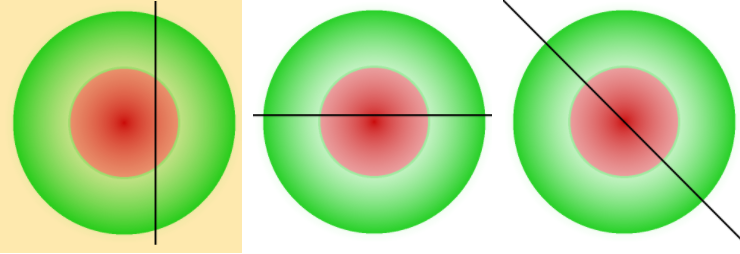
A linear model can separate places in original space only like:
To deal with this one can perform some feature engineering and find a way to project data into other spaces where data becomes more separable than initially. Let’s add a third dimension with squared distance from point to danger source:
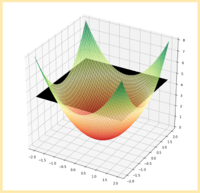
Now linear separation is possible – using a two-dimensional plane in three-dimensional space. In this simple example even usage of the only distance feature is enough to achieve linearity, in more complex tasks it is not so straightforward and the resulting space is as linear as possible, but not completely linear.
Many complex models can automatically learn projection from initial features space into new space, structure of such models include complex projection part and simple linear model over it. Proper training of such a model needs much more data than a simple linear model, though. So, when one works with machine learning, and real world data samples are not large enough, then a simple linear model is preferred over other options and besides model fitting also feature engineering is necessary.
Now, you are more familiar with some basic concepts. Time to look closer on computer vision specifics.
Computer Vision Specifics
Input for computer vision is images. Image consists of many pixels, even an image in poor resolution 320×240 has in total 76800 pixels. If we will just use all pixels as input to a machine learning model like logistic regression we will obtain a poor quality model due to lack of understanding of image semantics. Pixels one-by-one mean nothing, they are just pixels of different colors.
Image Features
To introduce more meaningful input for machine learning algorithms one needs to develop features: local (low-level) – values computed from a set of neighbouring pixels that have some underlying semantics, and global (high-level) – features somehow computed from local features. Trivial example of local features is color distribution in pixels near to corners. Global features can then be built as average or sum or element wise maximum of all local features.
Non-trivial universal example of such feature computation algorithms is SIFT – scale-invariant feature transform. It finds special key points on image and assigns for each of them a numeric descriptor (local features). Statistics of such descriptors (global features) then become input for machine learning models.
Any manual and specialized features computation algorithm is prone to both developer and their initial purpose induced biases and needs manual tuning for each new task. For example, if the algorithm considers corners as key points – it would not work on images without corners. Another and more promising way to compute features from pixels is to allow the model to learn such mapping by itself regarding needs of concrete problems. We may say that in this case the model will consist of two blocks – trainable feature extraction model and linear decision model (like linear regression). Well known example of such a combined model is artificial neural networks.
Artificial Neural Networks
Artificial neural networks are machine learning models initially invented as a simplified model of learning processes in the biological brain. Mathematically, one artificial neuron is not very different from the logistic regression model. It has input x, trainable weights w and bias b. Just alongside with sigmoid any other activation function usage is possible.
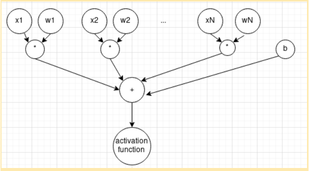
To build a neural network we have first to combine multiple neurons into layers and then stack multiple layers. Output of a layer is a combination of outputs from each neuron from the layer.
Outputs of different layers play the role of abstractions with similar semantic meaning. Usually we do not tweak it manually, we just believe it is so. Especially, for image processing we even know that first neural network layers after proper training become responsible for search of simple visual concepts – like lines and corners, later layers become responsible for more high level abstraction, and output layer is linear decision model-based on high level features. What we don’t know is what particular concept some neuron has from the deep part of the neural network describes. Layer which consists of linear neurons is called a linear or fully-connected layer.
In theory, even a neural network with a single trainable hidden layer (universal approximation theorem) is enough to split in finite time any data given a proper number of neurons on the hidden layer. In such a properly constructed network, its hidden layer will project data from input space to some intermediate space where initially non-separable data points will become separable. Output layer then just makes decisions based on transformed data points.
Why do we need to build deeper neural networks then? It is because the number of neurons on the hidden layer necessary to fulfill theorem conditions may be very large for real world tasks and training of such a network will need a great amount of memory and time.
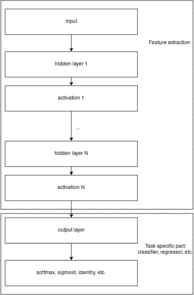
Most frequently used building blocks for neural networks for computer vision problem solving are: convolution layer, rectified linear unit, pooling layer, and softmax layer.
Convolution Layer
An usual RGB image is a three dimensional tensor of shape (W, H, 3). First two dimensions are spatial dimensions and the last (third) dimension is channel dimension.
Convolution layer performs transformation of input tensor, in particular input image, into new tensor of shape (Wout, Hout, Cout), where Cout – is number of convolution operations (neurons) on a layer, Wout and Hout are spatial dimensions of convolution operation output.
Convolution is in simple words the operation of applying the same fully connected layer to each spatial patch of given size of input tensor. If one mention convolution with kernel size 3×3, stride 1, input channels number Cin and output channels number Cout it means that each consequent (in spatial dimensions, with step size equal to stride equal to 1 here) patch of size 3×3 of input tensor goes as input of same neuron with trainable parameters (3x3xCin weights + 1 bias parameter) and become one pixel of output feature map. After applying Cout neurons all output feature maps are stacked into one output tensor. Direct application of convolution layer to tensor changes spatial dimension even if stride is set to 1. To handle this input tensor can be padded by zeros, so that output tensor spatial shape will match input tensor spatial shape – this is usual behaviour in most neural network architectures.
Saying simple, each convolution of convolution layer compares patches of input tensor with weights and outputs higher values where patch correlates with convolution weights.
ReLU Layer
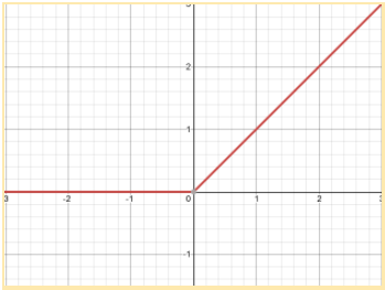
This layer transforms each its input by applying ReLU function:
ReLU (xi) = max {0, xi}
It is non-linear activation function which response to input signal is shown below:
Pooling Layer
Pooling layer performs spatial downsampling of input tensor. It leads to consequent transition from local features to global features. In particular, the max pooling layer transforms each non overlapping patch of input tensor of given size into one value equal to maximum value of the patch.
SoftMax layer
SoftMax layer applies SoftMax function to it’s input.

Like sigmoid, SoftMax compresses its inputs into an (0, 1) interval. The difference is that SoftMax does it so that all outputs sum up to 1, and we can see on it’s result as a discrete probability distribution.
Nowadays, any reasonable application of neural networks to computer vision problems is based on deep neural networks.
Deep Learning-Based Computer Vision
Deep Learning is a set of methods and tricks to train deep neural networks. Deep means, in general, that a network has more than one hidden layer – but in practice it is dozens of layers for modern neural network architectures.

Source: Unsplash
In recent years, Deep Learning (DL) has gained momentum in the computer vision community. The overall deep learning market is valued at USD 3.18 Billion in 2018 and is to reach USD 18.16 Billion by 2023, at a CAGR of 41.7% between 2018 and 2023, according to MarketsandMarkets.
Rosenblatt wrote that in 1958. And had a point. By that time, little did he know that he would develop a math algorithm to mimic the behavior of neurons in the human brain – the Perceptron.
BackPropagation (BP) was one more milestone for Artificial Neural Networks (ANN). BackPropagation is an algorithm for supervised learning using gradient descent. It was introduced in the early 1960s and first applied in 1974 by Werbos.
In 1989, LeCun used convolution operating instead of Pooling.
2 decades later, Hinton showed that Deep Neural Networks (DNNs) can achieve better results if the weights are better initialized. He rebranded the domain recently known as multi-layer NNs to Deep Learning (DL).
AI Revolution in Brief
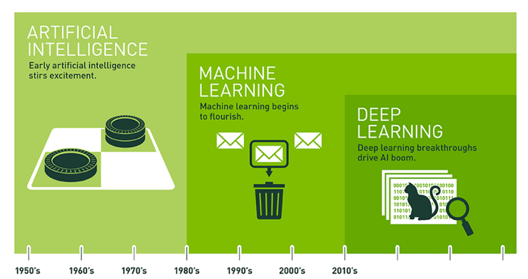
Source: xd.adobe.com/ideas
Up to 2021, deep learning success stands from:
- Computational device progress
- Underasting, how to train network more efficiently:
a) Activation functions with non-saturating (and even non-existing at some points) derivatives (like ReLU)
b) Feature normalization importance (batch normalization, layer normalization, group normalization)
c) Proper weights initialization methods
d) Neural network parameters factorization
e) End-to-end trainable network conception
f) Skip-connection conception
g) Fully convolutional network conception (this is especially important in computer vision area)
h) Data augmentation (also important in computer vision area) usage - Availability of automatic differentiation frameworks, allowing to create neural networks with stacking many of standard math operations without manual derivative computation, regardless of complexity of resulting function composition
Take a look and see how the technologies differ:
(a) Traditional Computer Vision workflow vs. (b) Deep Learning workflow
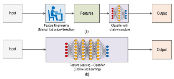
Source: Deep Learning vs. Traditional Computer Vision
Example of Deep Learning Architecture for Computer Vision
One of the first really deep architectures from which the rise of deep learning started is VGG [2014, https://arxiv.org/abs/1409.1556] architecture. Nowadays this architecture family is one of the simplest examples of modern deep learning architectures. Below we noted how image transforms passing through VGG-E architecture with 19 trainable layers.
| Layers block | Kernel size | Feature maps | Output of block |
|---|---|---|---|
| Input: | 224×224 RGB Image, 3 channels | ||
| Conv with ReLU, 2 times | 3×3 | 64 | 224×224 tensor, 64 channels |
| maxpool | 112×112 tensor, 64 channels | ||
| Conv with ReLU, 2 times | 3×3 | 128 | 112×112 tensor, 128 channels |
| maxpool | 56×56 tensor, 128 channels | ||
| Conv with ReLU, 4 times | 3×3 | 256 | 56×56 tensor, 256 channels |
| maxpool | 28×28 tensor, 256 channels | ||
| Conv with ReLU, 4 times | 3×3 | 512 | 28×28 tensor, 512 channels |
| maxpool | 14×14 tensor, 512 channels | ||
| Conv with ReLU, 4 times | 3×3 | 512 | 14×14 tensor, 512 channels |
| maxpool | 7×7 tensor, 512 channels | ||
| Classification subnetwork of flattening layer, three fully-connected layers and SoftMax | Vector of length 25088 (7x7x512) -> Vector of length 4096 -> Vector of length 4096 -> Vector of length 1000 -> Vector of length 1000 | ||
| Output: | Confidence level, that image belongs to one from given 1000 classes |
Research of deep learning and especially its application for computer vision from 2014 up to now gave us more complex models, computationally efficient models, smart network training tricks, and better accuracy for various computer vision problem solving. So, today, a computer vision specialist has many methods to start a particular computer vision project from.
Deep Model for Image Processing or Classic One?
Following table reflect our thought on both approaches to computer vision:
| Classic | Deep | |
| Generalization for out of lab conditions | Poor | Good |
| Simple explanation of model decisions and errors | Possibly | Only contradictory techniques exists |
| Quality | In general, poor | Deep models are SOTA for many tasks |
| Performance | Depends, but limited by feature extraction algorithm performance | Depends, but quality-performance tradeoff allows to get much faster models in cost of quality |
| Feature engineering phase | Essential | Not necessary |
| Quick prototyping | Possible, but expected quality is low without proper development efforts | Possible, often even with relatively good results |
| Train data needed | Not much | The more the better for quality |
| Actively developing area | No, part of history | Yes, each year gives many new problem solving methods and better understanding of whole deep learning area |
| Error in development cost | High (mostly human specialist time) | Low (mostly machine time) |
If one needs an interpretable model, even at the cost of quality and generalization ability, then deep learning is not a choice. Otherwise there is no reason to ignore deep learning.
Takeaway
Discoveries in deep learning have electrified the tech industry. Over the past years, we’ve seen quantum leaps in its quality. It’s leveled up computer vision, too. Сomputer Vision using Deep Learning allows for better application performance and accuracy. Moreover, it helps utilize the maximum of unstructured data. The data can come in different formats, but auctionable insights still can be gathered. And there more evidence to come that computer vision coupled with deep learning projects can achieve greater results.
Let’s Create Solid Computer Vision Solutions with Deep Learning
Need help to solve your business challenge? Contact our DL specialists at info@indatalabs.com.
